
Photon
numbers versus Telescope Diameter ---- or ----Where are all the photons
in an occultation experiment....
From Bessel (1979) PASP Vol91, pages 589-607 the following flux numbers can be derived for different photometric bands:
|
Band |
Center |
Flux m=0 [Jy] |
Flux in |
|
B |
0.44 |
4260 |
1.41 |
|
V |
0.55 |
3640 |
0.88 |
|
R |
0.64 |
3080 |
1.07 |
|
I |
0.79 |
2550 |
0.73 |
The unit is Jansky, 1 Jy = 10-26 W / (Hz m2). Depending on the wavelength the Flux can be converted to photons per second as given in the last column.
Example (without any atmospheric loss, no obstruction for secondary mirrors and no other optical loss) for a star with 15mag in each band results in the following photon numbers per second depending on telescope diameter:
|
Telescope diameter [m] |
B |
V |
R |
I |
|
1 |
11100 |
6900 |
8400 |
5700 |
|
0.6 |
4000 |
2500 |
3000 |
2100 |
|
0.5 |
2750 |
1700 |
2100 |
1400 |
|
0.4 |
1780 |
1100 |
1340 |
910 |
|
0.3 |
1000 |
620 |
760 |
510 |
|
0.2 |
440 |
280 |
340 |
230 |
Keep in mind, the unit is millions of photons per second!
More realistic numbers, what you have to expect on your CCD camera, you get in the following graph, it gives you an idea, what happens to all the photons from outside the atmosphere, up to the moment, they are absorbed in the CCD array. The integration time is assumed to be 0.5 seconds, the quantum efficiency of the chip including loss of the window is 0.3, the optical components of the telescope are reflecting 90% and the atmosphere transmits 60% of the flux.
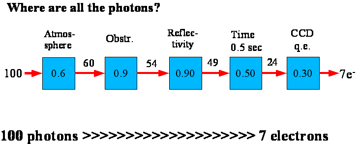
Therefore only 7 % of the above calculated photon numbers are registered as electrons in a typical occultation experiment. Taking the best possible values, we can have a quantum efficiency of about 90% for the chip, a reflectivity of 96% and 4% obstruction only. In this case we are getting about 50% of the photons into electrons. The reality may be somewhat in between.